Why I Built a Neural Network From Scratch

Today I did something I'd been putting off for a while: I implemented a feedforward neural network completely from scratch, using just NumPy and core Python, and trained it on MNIST to recognize handwritten digits. No model.fit(). No autograd. Every forward pass, every gradient, every weight update, written by hand.

And honestly? It clarified more about deep learning in one sitting than weeks of reading theory ever did.

I'd been avoiding it for a simple reason. Frameworks make it so easy to get a result that you can go a long time without noticing you don't really know what's happening underneath. You stack a few layers, call fit, watch the loss go down, and feel like you understand it. Then someone asks "wait, what does the backward pass actually compute?" and the confidence quietly leaves the room.

So I closed the framework docs, opened an empty Python file, and decided to build the whole thing myself. This post is the story of how that went: the architecture, the math I had to work out on paper, the three lines of code that made everything click, and the moment I watched it read my own terrible handwriting.

784 → 128 → 10architecture

101,770learnable parameters

0frameworks

The Problem: Teaching a Computer to Read Digits

The playground for this experiment is MNIST, the "hello world" of machine learning. It's a collection of 70,000 handwritten digits (60,000 for training, 10,000 for testing), each one a tiny 28×28 grayscale image. Every pixel is a number from 0 (black) to 255 (white), and every image comes with a label saying which digit from 0 to 9 it's supposed to be.

The task: given the 784 pixel values of an image, output which digit it is. To you, that's trivial. To a computer, an image is just a grid of numbers with no inherent meaning, and somehow it has to learn that a certain pattern of bright pixels means "7" while a slightly different pattern means "1".

The Architecture

Nothing exotic here. It's a simple 784 → 128 → 10 network:

Input layer (784): each 28×28 MNIST image flattened into a single vector. Row by row, the grid gets unrolled into one long line of 784 numbers.
Hidden layer (128): with a ReLU activation, ReLU(x) = max(0, x). This is the layer where the network builds its own intermediate features from raw pixels.
Output layer (10): one unit per digit, squashed through softmax to get class probabilities that add up to 1.

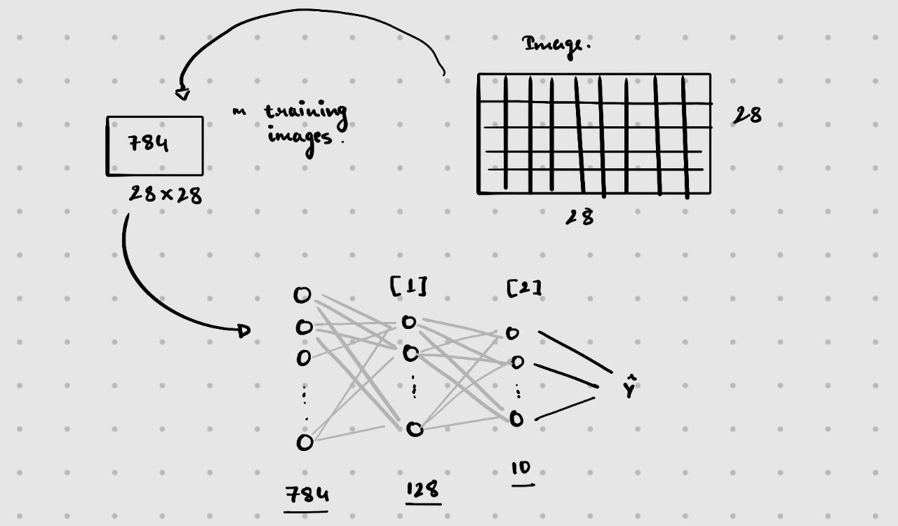
Hand-drawn sketch of the network: a 28 by 28 MNIST image is flattened into 784 inputs, which feed a hidden layer of 128 units and then an output layer of 10 units producing the prediction y-hat — My sketch of the whole idea: m training images, each flattened from 28×28 into a 784-long vector, flowing through 128 hidden units into 10 outputs.

A few quick words on why each piece is there:

Why flatten the image? A plain feedforward network expects a vector, not a grid. Flattening throws away the "these two pixels are neighbours" information, which is exactly why convolutional networks exist. But for digits, a plain network still does surprisingly well.

Why ReLU? Without a nonlinearity between layers, stacking them is pointless: two linear layers collapse into one. ReLU is the simplest nonlinearity there is (keep positive numbers, zero out negative ones), and that simplicity makes its gradient trivial too, as we'll see in a moment.

Why softmax? The last layer produces 10 raw scores (called logits) that can be any real number. Softmax exponentiates each one and divides by the total, turning them into 10 probabilities that sum to 1. Now the output reads as "I'm 93% sure this is a 4."

Counting the knobs

The first layer has 784 × 128 weights plus 128 biases (100,480 numbers). The second has 128 × 10 weights plus 10 biases (1,290 numbers). That's 101,770 parameters in total, and training is nothing more than nudging each of those numbers, over and over, in the direction that makes the predictions less wrong.

The Forward Pass

The forward pass is just four lines:

forward pass

Z1 = X @ W1 + b1
A1 = relu(Z1)
Z2 = A1 @ W2 + b2
P  = softmax(Z2)

Take the input, multiply by the first weight matrix, add a bias, apply ReLU, then repeat the same idea for the second layer and finish with softmax. That's the entire "thinking" part of the network.

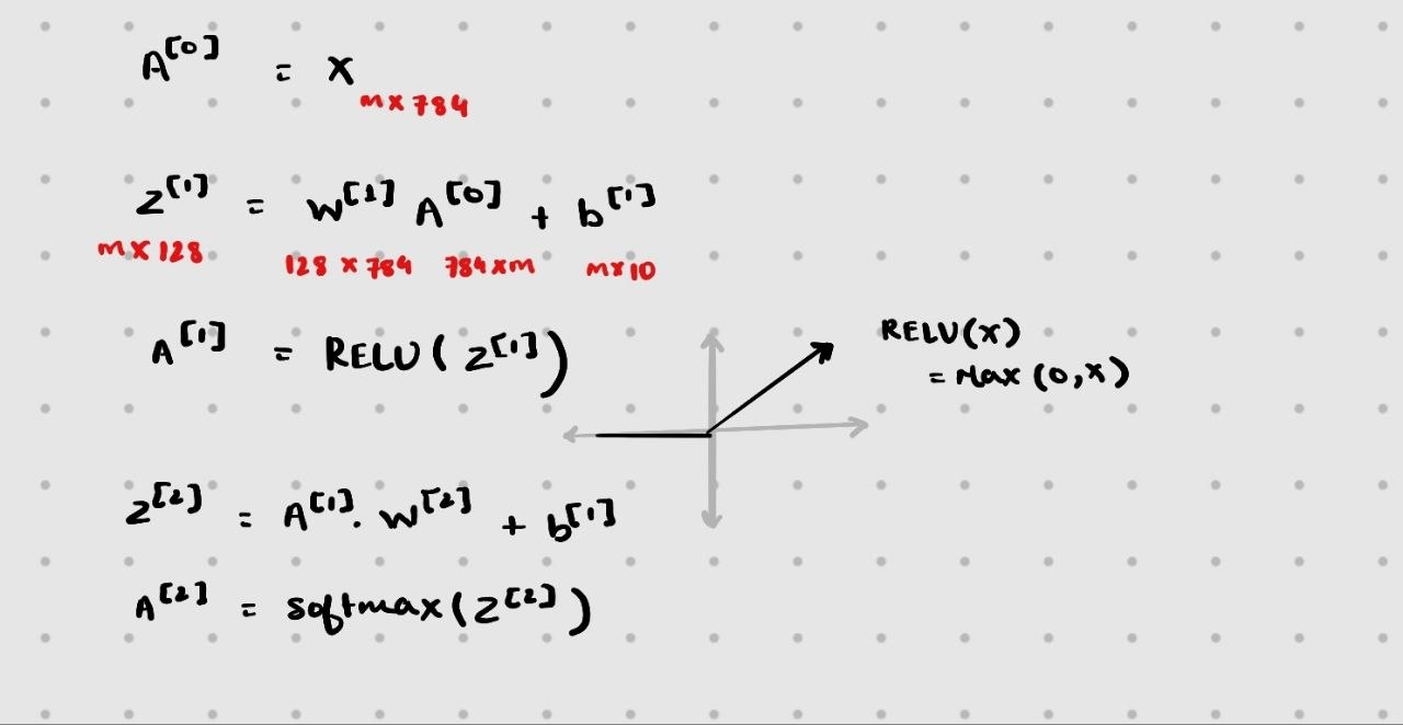
Handwritten forward propagation equations: A0 equals X, Z1 equals W1 times A0 plus b1, A1 equals ReLU of Z1, Z2 equals A1 times W2 plus b2, A2 equals softmax of Z2, with matrix dimensions annotated in red and a small plot of the ReLU function — The forward pass worked out by hand, with the matrix dimensions written in red. The little graph on the right is ReLU: flat at zero, then a straight diagonal line.

Simple to write. But writing it forced me to actually get the matrix shapes right, which sounds trivial until you're the one debugging a shape mismatch at 2am and realizing you transposed something three layers back.

Here's the shape bookkeeping for a batch of n images, which I ended up pinning to the wall of my brain:

Name	What it is	Shape
`X`	the batch of flattened images	n × 784
`W1`, `b1`	first layer weights and biases	784 × 128, 128
`Z1`, `A1`	hidden layer before / after ReLU	n × 128
`W2`, `b2`	second layer weights and biases	128 × 10, 10
`Z2`, `P`	output scores / probabilities	n × 10

One detail you might notice: my handwritten notes use the textbook convention W · A (each column is one example), while the code uses X @ W (each row is one example). Same math, transposed. It's a small thing, but it's exactly the sort of thing that bites you when you move from paper to code, and it's why I trust the shape table more than my memory.

How the Network Knows It's Wrong

Before it can improve, the network needs a single number that says how bad its predictions are. For classification, that number is the cross-entropy loss: for each image, look at the probability the network assigned to the correct digit, take the negative log of it, and average over the batch.

softmax: P_k = e^z_k / Σ_j e^z_j
loss: L = −(1/n) · Σ_i log P[i, correct digit]

The intuition is nice. If the network gave the right digit a probability of 0.99, then −log(0.99) is almost zero, so tiny loss. If it gave the right digit only 0.01, then −log(0.01) is huge, so it's punished hard. Confidently wrong is the worst place to be.

Where the Real Learning Happened: Backprop

Forward pass is the easy part. Backpropagation is where "I understand neural networks" turns into "I actually understand neural networks."

The goal is to find out, for every one of those 101,770 parameters, "if I nudge you up a tiny bit, does the loss go up or down, and by how much?" That's the gradient. Backprop is just the chain rule applied layer by layer, starting from the loss and walking backwards to the input, reusing work as it goes.

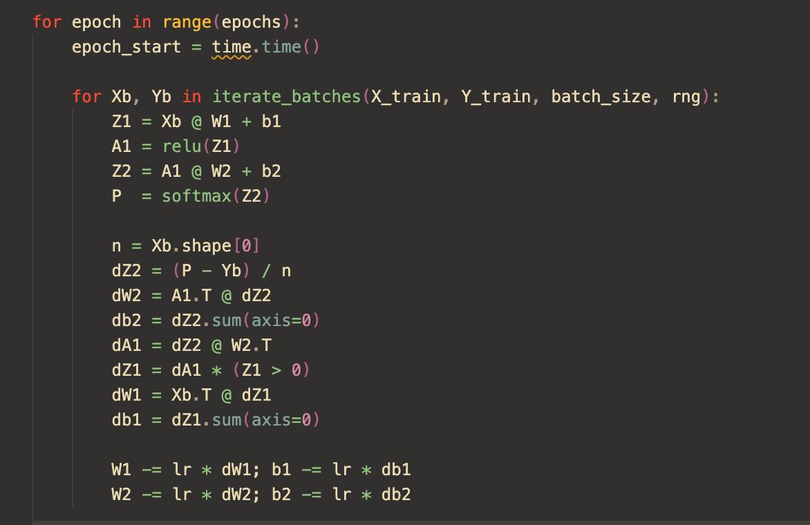
Deriving and coding the gradients by hand:

backward pass

dZ2 = (P - Yb) / n
dW2 = A1.T @ dZ2
db2 = dZ2.sum(axis=0)
dA1 = dZ2 @ W2.T
dZ1 = dA1 * (Z1 > 0)
dW1 = Xb.T @ dZ1
db1 = dZ1.sum(axis=0)

Read it top to bottom and you can feel the error flowing backwards: from the output scores dZ2, into the second layer's weights and biases, back through the weights into the hidden activations dA1, through ReLU into dZ1, and finally into the first layer's weights and biases. Each line is one link in the chain rule.

The line that made it click

That one line, dZ2 = (P - Yb) / n, is the softmax + cross-entropy gradient collapsing into something beautifully simple. When you've only ever called loss.backward(), that simplification is invisible. When you derive it yourself, it clicks: this is why softmax and cross-entropy are paired the way they are.

Softmax and the log in the loss each have a messy derivative on their own. Put them together and everything cancels down to prediction minus truth. Here Yb holds the correct answers as one-hot vectors (a 1 in the right column, 0 everywhere else), so P - Yb is literally "what the network believed" minus "what was true".

A tiny example

Say the image is an 8, but the network puts 70% on "3" and only 10% on "8". The gradient for the "3" score is 0.70 − 0 = +0.70 and for the "8" score it's 0.10 − 1 = −0.90. Gradient descent subtracts the gradient, so the "3" score gets pushed down and the "8" score gets pushed up. The size of each push is exactly how wrong the network was. No magic, just subtraction.

The / n is because the loss is an average over the batch, so each example contributes only a 1/n share of the gradient. Forget it, and your effective learning rate silently changes with your batch size.

ReLU as an on/off switch

Same with dZ1 = dA1 * (Z1 > 0): the ReLU gradient as a literal on/off mask. Where a hidden unit was active (Z1 > 0), the gradient passes straight through. Where it was off, the gradient is multiplied by zero and stops dead. Once you write that line yourself, "ReLU has zero gradient for negative inputs" stops being a fact you memorized and becomes something you can see in the code.

Matrix shapes as a sanity check

Here's a trick worth knowing: you can almost derive the gradient code just by making the shapes work. dW2 must be the same shape as W2 (128 × 10). The only way to get there from A1 (n × 128) and dZ2 (n × 10) is A1.T @ dZ2. Same story for dW1 from Xb.T @ dZ1. When the shapes only allow one answer, you can be much more confident it's the right one.

Putting It in a Loop

With gradients in hand, learning is one more step: move every parameter a small distance against its gradient.

weight update

W1 -= lr * dW1;  b1 -= lr * db1
W2 -= lr * dW2;  b2 -= lr * db2

lr is the learning rate, the size of each step. Too big and the loss bounces around or blows up; too small and training crawls. Around this update, the training loop has three ideas:

Mini-batches. Rather than computing the gradient over all 60,000 images at once, the data is shuffled and cut into small batches (iterate_batches in the code). Each batch gives a noisy but cheap estimate of the true gradient, and you get many updates per pass instead of one.
Epochs. One epoch is one full pass over the training data. The outer loop repeats this, and I time each epoch to see how long the whole thing takes.
The loop itself. Forward pass, backward pass, update, next batch. Thousands of times over. That's all "training" is.

There's something oddly humbling about it. The thing that eventually reads handwriting is those few lines of arithmetic, run over and over.

Then I Watched It Actually Work

After wiring up mini-batch training with a basic epoch loop, I didn't stop at a training-accuracy number in a terminal. I built a small "Draw a Digit" web interface where you draw a digit by hand and the network predicts it live, with a confidence bar chart across all 10 classes.

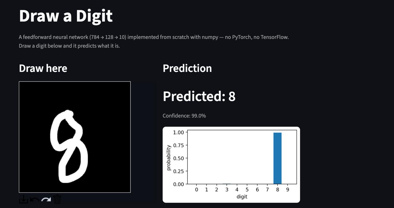
Draw a Digit web app: a hand-drawn white 8 on a black canvas, with the prediction shown as 8 at 99.0 percent confidence and a bar chart of probabilities across digits 0 to 9 with a single tall bar at 8 — My own messy 8, correctly read with 99.0% confidence. The bar chart on the right shows the probability the network assigns to each digit.

Notice the canvas is black with a white stroke. That's on purpose: MNIST digits are white on black, so to give the network input that looks like what it trained on, the drawing area has to look the same way. Your drawing gets shrunk down to 28×28, flattened into 784 numbers, and pushed through the exact forward pass from earlier.

Watching a network I built line by line correctly read my own messy handwriting, 99% confidence on an "8" I drew badly, hit different than any accuracy metric could. Look closely at the bar chart and you can even spot a barely visible sliver of probability on "3", which makes sense: an 8 is basically a 3 with the left side closed.

Things That Bite You When You Do This by Hand

If you try this yourself, here are the classic traps. Each one is invisible in a framework and very loud without one:

Shape mismatches. The number one error. When in doubt, print .shape at every step.
Forgetting to normalize the pixels. Raw values go up to 255, which makes the exponentials in softmax huge. Scaling to 0–1 keeps everything well-behaved.
Numerically unstable softmax. e to the power of a large number overflows. The standard fix is subtracting each row's maximum before exponentiating, which doesn't change the result but keeps the numbers small.
Initial weights that are too big or too small. If every weight starts at zero, every hidden unit learns the same thing. Small random values, scaled sensibly to the layer size, break the symmetry and keep signals a healthy size.
Wrong learning rate. A loss that explodes or refuses to move is almost always this.
Gradient bugs that don't crash. A wrong gradient still runs, it just trains badly. Comparing against a numerical gradient (nudge a weight, see how the loss changes) is the definitive way to check.

Why Implementing From Scratch Actually Matters

It's tempting to skip straight to high-level frameworks. They're faster, more robust, and let you ship things quickly. But there's a real gap between using an algorithm and understanding it. Frameworks abstract away exactly the details that make the ideas make sense: matrix shapes, gradient flow, why certain function pairs (softmax + cross-entropy) exist together.

Implementing from scratch forces you to confront every one of those details. You can't hide behind .fit(). Every bug is a conceptual bug, not a library-usage bug, and fixing it teaches you something durable.

A framework tells you that it works. Building it yourself tells you why.

This won't replace PyTorch or TensorFlow for real projects. Autograd exists for good reasons, and nobody should hand-derive gradients for a 50-layer network. But as a learning exercise, building the thing your framework of choice normally hides from you is one of the highest-leverage things you can do if you actually want to understand what's happening under the hood, not just call the right function.

If You Want to Try It Yourself

Load MNIST, flatten each image to 784 values, and scale them to 0–1.
Initialize W1, b1, W2, b2 with small random values.
Write the forward pass and check every shape.
Derive the gradients on paper first, then translate them to code.
Loop over shuffled mini-batches, updating the weights each time.
Draw your own digit and see if it recognizes it.

You'll get stuck, and that's the point. Every time you get unstuck, you'll understand something you can't unlearn.

References

I didn't figure this out in a vacuum. These are the resources I leaned on while building it, and I'd recommend all of them:

Building a Neural Network From Scratch by Samson Zhang (YouTube). A walkthrough of building a network with only NumPy and math, the video that got me started.
The Math Behind Neural Networks (Towards Data Science). The written derivations I checked my gradients against.
An Introduction to Statistical Learning with Applications in Python (ISLP) by James, Witten, Hastie and Tibshirani. I borrowed from its code examples for parts of my implementation.